How to freeze header data in Excel?

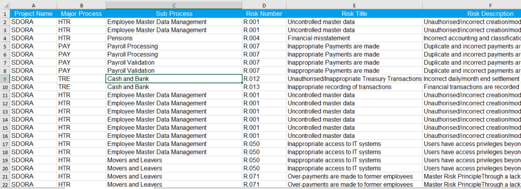
When you are working on big excel data and when you move your cursor from one column to another or from one row to another row, you might have faced difficulties with viewing header row data.

Here we will see how we can freeze our excel header data, so that while moving from one cell to another cell at the bottom then you will see the header data.

Step – 1

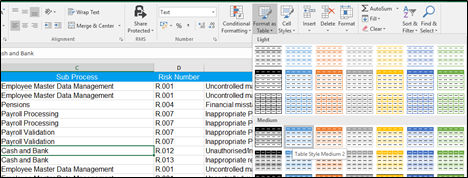
Select any cell in the data and then Select Home > Format as Table

Step- 2

Select any Table Style from “Format as Table Tab”

Step- 3

Once you click any Table Style from “Format as Table Tab“, Excel will select the whole data, and one pop up will come i.e. “Format As Table“. Once the pop up comes then click to the “Ok” button.

Step-4

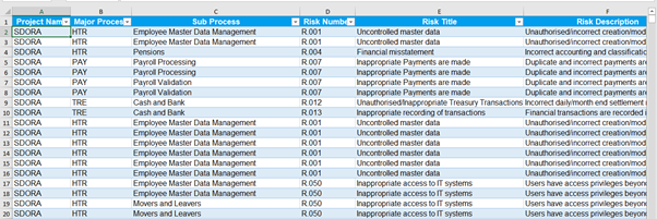
Excel will change the colour of the data and header data will freeze along with “Filter”

Now wherever you move your cursor within the data you will see the header level information with a filter. This helps you to understand on which column you are working

Advantage-

1. Utilization of least organizing with no time
2. No need to go for Freeze pane
3. Customize the function from the drop-down list

Use this little handy feature to have the headers visible when you scroll and always know what figures you are looking at.

Follow me

• 
• 
• 
• 
• 
•